Table of Contents |
|---|
Figures | |
|---|---|
| 
|
| 
|
| 
|
| 
|
| 
|
|
|
Beshers, C. and Feiner, S. AutoVisual: Rule-based design of
interactive multivariate visualizations.
IEEE Computer Graphics and Applications,
13(4), July 1993, 41-49.
For n-Vision, we invented a method of composing graphs we call worlds within worlds. Rather than inventing subtle ways of mapping information to geometry and color, we create interactive worlds composed of standard graph types, e.g., surface plots and line graphs. Worlds within worlds is a powerful method, capable of displaying many dimensions, and yet is readily understandable.
Although this simple approach effectively slices away the higher dimensions, it is possible to add them back. To do this, we embed the 3D world in another 3D world. The position of the embedded world's origin relative to the containing world's coordinate system specifies the values of up to three variables that were held constant in the process of slicing the world down to size. This process can then be repeated by further recursive nesting.
We allow the user to create these virtual worlds by specifying the assignment of variables to coordinate system axes. We can deposit multiple copies of the same world, or copies of different worlds within a containing world, to allow the copies to be compared visually. Each copy has a different constant set of values of the containing world's variables, based on its position. Worlds may be rotated and scaled about their origins, and viewed from different positions.
f(x1,x2,x3,x4,x5).Following the description above, we first select constant values for three variables x3,x4,x5, call them c3,c4,c5. This selection results in a new function f':
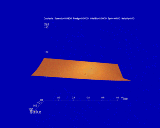
f'(x1,x2) = f(x1,x2,c3,c4,c5).The function f' is easy to graph in 3D as a surface plot, with x1 on the X-axis, x2 on the Z-axis, and the value of the function on the vertical axis (Y-axis). This graph is shown in the Figure 1; it is the smaller of the two graphs. To let the user select particular values for x3, x4 and x5, we graph them on a separate set of axes, bound to the X, Y and Z axes respectively. Selecting a point within this larger graph determines the particular values of c3, c4 and c5 used in the smaller graph. Thus, the contents of the smaller graph depend on the location of some interactive mark in the larger graph.
We represent this dependency explicitly by attaching the origin of the smaller graph (the surface plot) to the interactive point in the larger graph. To change the values of x3, x4 and x5, the user grabs the surface plot and translates it relative to the larger world. That is, the surface plot is nested within the graph of x3, x4 and x5.
We call the dependent world (with the surface plot) an inner world, i.e., it is nested within the other world. Accordingly the larger world is called the outer world. This is important because the worlds may be scaled such that the outer world is actually smaller than the inner world.
Only the position of the origin of the inner world relative to the outer world affects the values of c3, c4 and c5, and hence the values displayed in the surface plot. Both the inner and outer worlds may be scaled and rotated for better viewing. In addition, translation of the outer world may be used to give a better view, without affecting the contents of the graph.
Follow for high resolution
Figure 1. An n-Vision world that encodes a function of five variables as a hierarchy of graphs. The height field in the inner world encodes the function for constant values of x3, x4, and x5, determined by the position of the inner world's origin relative to the outer world. As the user translates the inner world, n-Vision updates the height field. A one-dimensional graph, called a dipstick tool, provides a precise readout at one point of the height field.
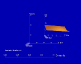
At the bottom right is a zoom tool, which displays a scaled up view of a selected world. The graph of the parent world is redisplayed within the zoom tool. The zoom tool is an example of a world that can be detached from the world it depends on, making it possible to get the best viewing without disturbing the existing worlds.
Follow for high resolution
Figure 2. An n-Vision virtual world showing a line graph tool and a zoom tool in use. The line graph tool redisplays a univariate subset of the height field, and may be aligned with either horizontal axis. The zoom tool redisplays the contents of a world. A box is drawn around the world being redisplayed.
We define an n-Vision virtual world as a hierarchy of interactors. Each interactor consists of four basic components: a set of encoding spaces, a set of encoding objects, a set of selections, and a user interface.
An encoding space is a region where the graph is rendered. In general, an encoding space may be of any dimension (up to three), arbitrarily positioned and oriented in the 3D world. Many interactors have constrained placement; for example, the encoding space of the dipstick is a line constrained to be within the encoding space of the parent world and parallel to its vertical axis. An interactor may have multiple encoding spaces; for example, to provide redundant encodings of the same relation using different encoding methods.
The set of encoding objects comprise the body of the graph (e.g., a height field). An interactor may have no encoding objects, as in the outer world of Figure 1. The potential set of encoding objects includes essentially any known visualization technique.
A selection determines the relation encoded by the interactor. It consists of a geometric subset of the encoding space of the parent interactor. This geometric subset determines a subset of the relation encoded by the parent. The selection may be any axis-aligned rectangular volume of a dimension less than or equal to that of the parent encoding space. For example, the selection component of the height field interactor is a point (typically the inner world's origin) in the coordinate system of the outer world. An interactor may have multiple selections, such as a comparison tool that redisplays several parent interactors in one space.
Finally, the user interface component of an interactor consists of bindings between user actions and properties of the interactor. For example, the height field world has bindings for translation, scaling, and orientation in 3-space. In contrast, the dipstick only has bindings for translation, because its size and orientation are determined by its parent. Each interactor has bindings for creating, copying, and deleting child interactors.
Exploration has the form explore(S), where S is a task selection (described below). An appropriate visualization provides a summary reading, allowing the user to view the entire selection as quickly as possible. A user would typically choose exploration if the relation is unfamiliar.
Directed search has the form search(Sgoal,Scontext), where Sgoal and Scontext are both task selections. Sgoal union Scontext forms the complete context (i.e., the set of variables that should be considered for binding to axes). If Scontext is omitted, the context is the entire relation. An appropriate visualization allows the user to adjust the variables in Scontext and clearly view the effect on Sgoal. This makes it possible to search for a subset with a particular characteristic.
Comparison has the form compare(S1, ..., Sk), where k >= 2. The visualization must allow comparison to be done easily, ensuring that all selections are encoded in the same space (or perhaps juxtaposed spaces), and that all encodings are visible. The task is to study the relationship between selections.
The variable names are included in the notation so that the restrictions may be specified in any order. Besides being convenient, this allows the user to order the variables. A switch lets the user override AutoVisual's variable priorities, substituting the order from the task selection. In addition, any omitted variable is assumed to have the default constraints.
Our first domain involves calculating monthly payments for a conventional fixed-rate mortgage. The function to compute the monthly payments has the form: mortgage(i,P,D,T,I,t), where i is the interest rate, P is the price of the house, D is the down payment, T is the monthly property tax, I is the monthly insurance, and t is the term or duration of the loan in years. Both P and D are in units of thousands of dollars.
Potential home buyers need to understand the limits and tradeoffs on their finances. For example, before searching for houses, realtors recommend finding an approximate maximum affordable price, assuming a conventional 30 year mortgage. To do this, home buyers need to see the effect of house price and down payment on the monthly mortgage. Thus, they have the following visualization task:
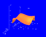
explore(mortgage(P[-],D[-], t[30])).Figure 3 shows the visualization produced by AutoVisual. The height field presents a complete summary of the selection, while the line graph tool displays a subset whose values can be read more precisely.
Follow for high resolution
Figure 3. An n-Vision world that encodes a function of five variables as a hierarchy of graphs. The height field in the inner world encodes the function for constant values of x3, x4, and x5, determined by the position of the inner world's origin relative to the outer world. As the user translates the inner world, n-Vision updates the height field. A one-dimensional graph, called a dipstick tool, provides a precise readout at one point of the height field.
Suppose now that a potential home buyer has been looking at houses and wishes to examine the finance options for each, knowing that they can make a down payment of $10,000. For each house, the price, taxes, and insurance are fixed. Because banks do not offer arbitrary interest rates and terms, the buyer is interested in particular values, not ranges. An appropriate visualization task might be:
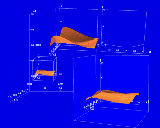
search(mortgage(t[?],i[?]),mortgage(P[?],T[?],I[?],D[10])).Figure 4 shows the visualization that has been created. The height field shows the goal selection, and the dipstick allows individual values to be read exactly. Particular houses are considered by positioning the inner world.
Follow for high resolution
Figure 4. Visualization generated for the mortgage search task. The visualization allows the user to set the price, property tax and insurance values for a particular house, and view the resulting mortgage payment as a function of the interest rate and the down payment. The line graph tool shows the payment as a function of the interest rate for a particular down payment.
Our second domain uses the Black-Scholes formulae for computing the value of a European foreign currency option [Hull]. A European option is a contract that gives the holder the right (but not the obligation) to buy or sell something at a specific price ( striking price) on a specified date ( maturity date). In this case, foreign currency is being bought or sold. An option to buy is referred to as a call, while an option to sell is referred to as a put. A function to compute the Black-Scholes formula for a European foreign currency call option has the following form: call(S,sigma,t,K,id,if,M), where S is the current ( spot) trading price of the currency, sigma is the standard deviation ( volatility) of S over the previous year, t is the time (date), K is the striking price, id and if are the risk-free interest rates in the domestic and foreign markets respectively, and M is the maturity date. M is in units of years and is normalized so that 0 represents the creation date of the contract. The value of t varies between 0 and 1, representing the fraction of contract time that has expired. Each of these is specified with a default value and range. The function to compute the put option has identical parameters.
A logical first step in understanding any relation is to get an idea of its overall behavior. Thus, one task is to explore the value of a call option for fixed maturity:
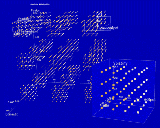
explore( call(S[-],sigma[-], t[-],K[-], if[-],id[-]) ).The resulting visualization is shown in Figure 5. This display shows the value of the function, represented as a color, with respect to six variables. The presentation is coarse, but general trends can be distinguished. A line graph tool and zoom tool have been included to aid in viewing and understanding the visualization. Since the line graph is sampling a point cloud, unlike the line graph tool of Figure 2, it has two degrees of freedom and samples along the horizontal line extending from its base.
Suppose we would like to analyze call options in more detail. We note that the variables S, sigma, id and if represent market conditions, while K and M are features of the option contract. Thus, two questions that are commonly asked are:Follow for high resolution
Figure 5. Visualization generated for exploring a call option. AutoVisual chose the point cloud interactor because it encodes many variables. The hierarchy is populated with point clouds so that the visualization presents a summary of the function, with little or no interaction required by the user. The zoom tool can be used to examine the point clouds. The line graph tool redisplays a portion of a point cloud using a superior encoding technique.
The first question corresponds to the task:
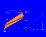
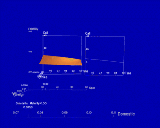
search( call(t[-],K[-]), call(S[?],sigma[?],if[?],id[?]) ).AutoVisual generates the world shown in Figure 6. Note that this hierarchy has three levels of worlds. The outermost 1D world encodes only the domestic interest rate. As in Figure 4, a height field encodes the goal selection. Note that if a point cloud were selected, there would be only one outer world, not two. Generally, it is desirable to have fewer levels, but AutoVisual gives priority to encoding the goal selection in a search task.
For the second question, we specify the task:Follow for high resolution
Figure 6. Visualization generated for the first option search task. The goal selection is encoded as a height field. Note that if AutoVisual had selected a point cloud as the encoding technique, the hierarchy would have only two levels.
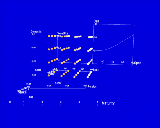
search( call(S[-],sigma[-],t[-],if[-],id[-]), call(K[?],M[?]) ).The resulting visualization is shown in Figure 7. The first three variables in the goal selection are encoded by a point cloud. Because the goal selection has so many variables, AutoVisual could not encode it with a single interactor, as in the previous task.
Suppose we would like to see how the put and call options differ. Our task would be to compare the two options under identical conditions:Follow for high resolution
Figure 7. Visualization generated for the second option search task, the search for market conditions. The goal selection is too large to be encoded with a single interactor. AutoVisual selected the point cloud because it encoded the most variables.
compare(call(S[-],sigma[-],t[-],K[-],if[-]), put(S[-],sigma[-],t[-],K[-],if[-])).
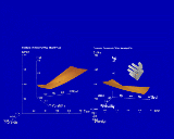
The generated visualization is shown in Figure 8. Note the parallel structure between the two hierarchies. The inner worlds translate in tandem, assuring that the inner worlds have corresponding values. However, the user may rotate and scale them independently to adjust the view. A representation of the user's hand appears at the upper right of the figure.
Follow for high resolution
Figure 8. Visualization generated for the option comparison task. The two hierarchies are designed to have parallel structure, and the inner worlds are constrained to move in tandem, so that visual comparisons may be made easily. However, the inner worlds may be rotated independently to get the best view of each.
In AutoVisual's search strategy, each state represents a possible interactive visualization world and is a directed acyclic graph of interactors. The state change operators simply add interactors or modify those already in the graph, producing the final visualization by incremental refinement. When necessary, backtracking is employed to undo a design path that proves to be unsuccessful. The selection of operators is driven by a rule-base of visualization design principles, taking into account the task to be performed, the interactors available, and the capabilities of the current hardware.
Termination conditions are a necessary part of any search algorithm. AutoVisual uses two criteria to establish that it has found a satisfactory visualization: potential expressiveness and potential effectiveness. These are Mackinlay's expressiveness and effectiveness criteria, modified for interactive visualization. An expressive graph encodes all relevant information and only that information. An effective graph presents that information clearly. We say that an interactive visualization is potentially expressive, if it has the potential, under user control, to display all its assigned information over time. Similarly, an interactive visualization is potentially effective if its use over time can present the information sufficiently clearly. (Note that no single static view need be sufficiently effective and expressive by itself for the visualization to be potentially expressive and potentially effective.)
For example, consider a task we used earlier, the search for option parameters that yield high profits:
search(call(t[-],K[-]), call(S[?],sigma[?],if[?],id[?])).AutoVisual begins the first phase by establishing a priority order among the relation variables. This ordering determines the assignment of variables to axes. For any search task, variables in the goal selection are always of higher priority than those of the context. In this example, we assume that the user has explicitly established the order within each selection. Thus, the overall priority of variables is t, K, S, sigma, if, id.
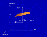
The next step is designing the main hierarchy, beginning with the innermost world, and proceeding outward. For this task, a height field is selected as the primary encoding object for the innermost world, because it encodes the entire goal selection effectively. The value of the relation is bound to the vertical axis, and the two variables of highest priority, t and K, are bound to the horizontal axes. Figure 9 shows the partial design at this point. Next, the remaining variables are recursively bound to outer worlds, as shown in Figure 10. A 3D world is created for S, sigma, and if, and an outermost 1D world is created for id.
Follow for high resolution
Figure 9. The design process begins with the choice of an encoding object and relation variables for the innermost world. This figure shows an incomplete visualization of the search for good option parameters after this stage. The parameters t and K form the goal selection and hence have high priority. The height field is selected because it encodes the entire goal selection effectively enough for the search task.
In the final step of the first phase, AutoVisual selects tools to examine the innermost worlds. These tools ensure that the user can find an accurate encoding of any value. AutoVisual considers as candidates those tools that encode fewer variables than the encoding object of the innermost world. Since the height field encodes two variables, the acceptable tools for this world are the dipstick and the line graph. Both allow reliable elementary readings. However, the dipstick has two degrees of freedom in the horizontal plane of the inner world, whereas the line graph has only one. AutoVisual chooses the line graph tool because it achieves the same goal with few degrees of freedom.Follow for high resolution
Figure 10. After the innermost world has been selected, outer worlds are added recursively until all variables have been bound. This figure shows the incomplete visualization for the search for good option parameters after this step has been performed. The final visualization is shown in Figure 6.
AutoVisual next enters the instantiation phase, in which it determines how many instances of each interactor type to create, and adjusts attributes such as position, size, and color. At least one of every type of selected interactor is created as a way of documenting the structure and capabilities of the world. The result is the world shown in Figure 6.
The design process is similar for exploration and comparison. For comparison, the design process is repeated for each selection, except that most of the decisions are forced to be the same as those made for the first selection, ensuring that all the worlds have a similar structure to aid in visual comparison.
Recall that an interactive visualization is potentially effective if its use over time can present the task information sufficiently clearly. To achieve this, at least these three criteria must be met: the encoding techniques must be effective, the amount of interaction required should be minimal, and the visualization should have low response time. Unfortunately, it is often the case that the more a visualization satisfies any one of these criteria, the less it satisfies the other two. For example, increasing the sampling rate of an encoding object can improve its effectiveness at the expense of increasing its computation and rendering time.
To ensure that the composition of interactors is effective, AutoVisual must consider their 3D spatial relations as well. Interactors that are too large may intersect, disrupting each other's presentation. Interactors that are too tightly packed may be hard to view. Even if interactors do not intersect in the world, their projections may intersect on the viewplane. If this occurs, opaque encoding objects can obscure each other, while transparent encoding objects or point clouds can make poor backgrounds for each other. Finally, all interactors must be easily viewable against the background.
Rendering time can be controlled by choosing encoding objects that are faster to render, possibly compromising the effectiveness of the presentation. While AutoVisual has no control over the evaluation time for a single sample, it can vary the number of samples calculated to generate the encoding objects. Since interactors only resample the relations when their selections move, it is also possible to trade rendering time for evaluation time by pre-sampling many values when the hierarchy is created, as in Figure 5, created for option exploration task.
This work is supported in part by the New York State Center for Advanced Technology under Contract NYSSTF-CAT-92-05, the Center for Telecommunications Research under NSF Grant ECD-88-11111, NSF Grant CDA-90-24735, ONR Contracts N00014-91-J-1872 and N00014-94-1-0564, and an equipment gift from the Hewlett-Packard Company. Early work on n-Vision was also supported by a gift from Citicorp.